The Model on Your Laptop

Like a lot of developers lately, I have a low-grade anxiety about keeping up with AI. There is a new model or framework or technique almost every week, and more evenings than I would like to admit end up on YouTube trying to catch up on whatever I missed. The thing I kept hearing about was running language models locally: not calling someone else’s API, but downloading the model itself and running it on your own machine. So one evening I actually tried it. I grabbed a small Qwen model, a few hundred megabytes on disk, ran a single command, and typed a question. Text streamed back a few hundred milliseconds later. No API key, no per-token bill ticking up in a dashboard somewhere, and once the file was downloaded, no network involved at all.

The surprising part was not that it worked. It was how small the model was. Under a billion parameters, a file smaller than a music album, and it still held a coherent conversation. For years the mental model most of us carried was that “real” language models live in a data center, behind an API, on hardware you will never touch. That is still true for the largest ones. But the floor has dropped. A model you can fit in memory on a mid-range laptop is now good enough to be genuinely useful, and the tooling to run it has quietly become excellent.

The tool that made running that model a one-liner is llama.cpp. It is an open-source inference engine written in C and C++ that loads a model file and runs it directly on your own hardware: your CPU, your GPU, your laptop’s memory. No server round-trip. The model lives on your disk and runs in your process. That is the entire premise, and this article is about understanding it from the ground up.

In this article, we are going to build up the full picture, one layer at a time. We will start with what a language model actually is and how it produces text. We will look at the difference between open and closed models, and why you would run a small open one locally at all. Then we get into the two ideas that make local inference practical: quantization (shrinking the model) and the KV cache (making it fast). We will cover GGUF, the file format llama.cpp uses, and how it relates to the other formats floating around Hugging Face. After that it is hands-on: installing llama.cpp on an Apple M2 Pro, running your first model from the command line, understanding chat templates and sampling, launching the HTTP server, and finally calling the whole thing from TypeScript, both over HTTP and in-process.

What we are not covering: training a model from scratch, fine-tuning an existing one, serving models across a cluster of GPUs, or anything about building AI agents on top of these models. Those are large topics in their own right, and I will link the official documentation where they come up, starting with the llama.cpp documentation itself if you want the canonical reference alongside this article. This is a pure “how do I run a model on my own machine, and what is actually happening when I do” explainer. Everything here is written against an Apple M2 Pro, which uses Apple Silicon with unified memory and the Metal GPU backend, but the concepts carry over to any machine.

Let’s start with the thing in the middle of all of this: the model.

---

How a Language Model Actually Works

Before we can run a model, it helps to know what the file on your disk actually contains and what happens when you give it a prompt. You do not need the math. You do need the mental model, because almost every flag and setting later in this article is a knob on one of the mechanisms described here.

What a model is

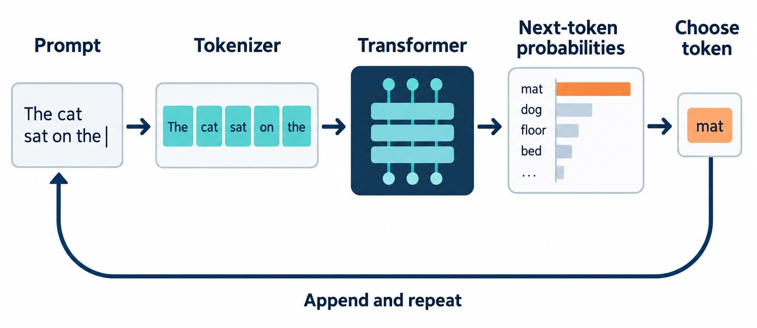
At its core, a language model is a next-token predictor. You give it some text, and it produces a probability distribution over what the next chunk of text should be. That is the whole job. It does not “know” things the way a database does. It has absorbed statistical patterns from an enormous amount of text, and it uses those patterns to guess what comes next, over and over, one chunk at a time.

Think of it like the autocomplete on your phone keyboard, except instead of suggesting the next word from a tiny built-in dictionary, it is drawing on patterns learned from a significant slice of the written internet. Your phone suggests “morning” after “good”. A language model, given “The capital of France is”, assigns a very high probability to “Paris” because that sequence appeared countless times in its training data. Generating a full answer is just doing this prediction step repeatedly, feeding each predicted chunk back in as part of the input for the next prediction. One detail to flag now: each step only yields that probability distribution, and a separate step still has to pick one token from it, whether by always taking the most likely or by rolling a weighted die, which is the choice we will later tune under the name sampling.

The transformer, briefly

Nearly every modern language model is built on an architecture called the transformer. You will see the word everywhere, so it is worth a plain-language definition even though we will not touch the math.

The transformer exists because the designs that came before it read text strictly left to right, one word at a time, and struggled to connect words that sat far apart in a sentence. The transformer instead weighs every word against every other word at once, which captures long-range meaning and, as a bonus, makes training parallelizable rather than strictly sequential.

A transformer is a stack of identical layers. Text enters at the bottom as a list of numbers, flows up through the layers, and a prediction comes out the top. The key trick inside each layer is attention: a mechanism that lets the model, when processing one piece of text, look back at every other piece of text it has seen so far and decide which ones are relevant. When the model is predicting the word after “The trophy did not fit in the suitcase because it was too big”, attention is what lets it work out that “it” refers to the trophy and not the suitcase. Each layer refines this understanding a little more, and a model has anywhere from a couple dozen to over a hundred of these layers stacked up.

That is as deep as we need to go. The one thing to hold onto is that attention looks back at everything so far. That single fact is why the KV cache (which we will get to) exists, and why memory usage grows as your conversation gets longer.

Parameters and weights

When you see a model described as “0.6B” or “7B”, that number is its parameter count. A parameter, also called a weight, is a single number that the model learned during training. “0.6B” means roughly 0.6 billion numbers. “7B” means 7 billion. These numbers are the model. They are the knobs that attention and every other part of the network use to turn input text into output predictions.

Why does this matter so much for running a model locally? Because every one of those numbers has to be held in memory while the model runs. If each parameter is stored as a 16-bit number (2 bytes), a 0.6B model needs about 1.2 GB just to hold its weights, and a 7B model needs about 14 GB. This is the single biggest factor in whether a model will fit on your machine, and it is the entire reason quantization (shrinking those numbers) exists. We will do the exact memory arithmetic later, but the relationship is simple: more parameters means a bigger file and more memory, which usually means a smarter model that is harder to run.

Tokens and tokenization

A model does not actually read text as letters or words. It reads tokens. A token is a chunk of text, often a whole short word, sometimes a word fragment, sometimes a single character or a space. Before any text reaches the model, a component called the tokenizer splits it into these chunks and maps each one to an integer ID. The model only ever sees those integers. When it produces output, it emits token IDs, and the tokenizer maps them back to text.

Why chunks instead of words? Because a fixed dictionary of whole words could never cover every name, typo, URL, and made-up term the model might encounter. By breaking text into sub-word pieces, the tokenizer can represent literally any string, even one it has never seen, by assembling it from smaller known pieces. The word “tokenization” might become token + ization, two tokens. A rare word gets split into more pieces, a common word stays whole. Think of it like building words out of LEGO: a common word is a single large pre-moulded brick, while a rare or novel word is assembled from several smaller standard pieces that can combine into anything.

💡 This is why usage and context limits are measured in tokens, not words. A rough rule of thumb for English is that one token is about four characters, or roughly three-quarters of a word, so 1,000 tokens is around 750 words. Code and non-English text often tokenize less efficiently, meaning more tokens per visible character.

Tokenizers also define special tokens: reserved IDs that do not correspond to ordinary text but to structural markers. These include things like a start-of-sequence marker, an end-of-sequence marker that signals the model is done generating, and the role markers used in chat formatting. We will see these special tokens become very important when we get to chat templates, because getting them wrong is one of the most common reasons a local model produces garbage.

Training vs inference

There are two completely separate phases in a model’s life, and keeping them straight clears up a lot of confusion. Training is the process of learning the parameter values in the first place: feeding the model enormous amounts of text and slowly adjusting all those billions of numbers until its predictions get good. This is astronomically expensive, requiring clusters of specialized hardware running for weeks or months, and it is done once by the organization that releases the model.

Inference is using the already-trained model to generate text. You load the fixed parameters, feed in a prompt, and the model produces output. Inference is far cheaper than training, cheap enough to run on a laptop, which is the only reason any of this is possible locally. When you run llama.cpp, you are doing inference and only inference. The parameters never change. You are not teaching the model anything; you are asking an already-educated model questions.

The cost of inference is not zero, though. Every token the model generates requires one full pass through all those layers, touching a large fraction of those billions of parameters. That is why generation speed is measured in tokens per second, and why a bigger model that must touch more parameters per token generates text more slowly. Training built the model; inference is what you pay for every time you use it. If you want to go deeper on how training and fine-tuning actually work, the Hugging Face course is a solid starting point, but we are leaving both behind from here on.

---

Open Models vs Closed Models

Now that we know what a model is, the next question is a practical one: which models can you even get your hands on to run locally? This is where the line between open and closed matters, and the terminology is muddier than most people realize.

What “open” means

When people say a model is “open”, they can mean three different things, and conflating them causes real confusion. Open weights means the trained parameter file is published and you can download it and run it yourself. Open source, in the strict sense, would additionally mean the training code and the training data are published so you could reproduce the model. Open license is about what you are legally allowed to do with it: use it commercially, redistribute it, build products on it, or only tinker with it for research.

Almost every “open” model you will run locally is open-weights with a permissive-enough license, but not fully open-source in the reproduce-it-from-scratch sense. The weights are the thing that matters for running the model. You download the file, llama.cpp loads it, and you are off. Whether the training data was published rarely affects you as someone just trying to run inference.

💡 Always check the license of a model before using it in anything that ships. Some popular open-weights models carry restrictions on commercial use, on using their output to train other models, or on use above a certain scale. The weights being downloadable does not automatically mean you are free to do anything you want with them.

The closed frontier

The most capable models in the world right now are closed. ChatGPT (from OpenAI), Claude (from Anthropic), and Gemini (from Google) are hosted services. You never see the weights. You send text to an API, it runs the model on their hardware, and it sends text back. These models are enormous, far larger than anything you could run locally, and they are kept behind an API both to protect the investment that went into them and because almost nobody has the hardware to run them anyway.

The tradeoffs are the obvious ones. You get the best quality available and zero infrastructure to manage, in exchange for a per-token cost, a hard dependency on an internet connection, and the reality that your prompts leave your machine. For many tasks that trade is worth it. For some, it is not, and that is where local models come in.

The open field

The open-weights world has become genuinely rich. A handful of families cover most of what you will encounter. Qwen (from Alibaba) is a broad family with excellent small models, and it is what we will use throughout this article. Llama (from Meta) is the family that started the local-model wave and gave llama.cpp its name. Gemma (from Google) is the open sibling of the closed Gemini line. Mistral (from the French lab of the same name) is known for strong, efficient models. DeepSeek made waves with strong reasoning models. Phi (from Microsoft) specializes in small models trained on carefully curated data.

These families each release models at a range of sizes, often from under a billion parameters up to tens of billions. The small end of each family (anything under a few billion parameters) is what fits comfortably on a laptop. The large end needs serious hardware. For local use on a machine like an M2 Pro, you live at the small end.

Why run a small open model locally

So why would you deliberately run a smaller, less capable model on your own machine instead of calling a frontier API? There are five honest reasons. Privacy: the text never leaves your device, which matters for sensitive data, regulated industries, or just personal preference. Offline: once the model is downloaded, it works on a plane, in a basement, or anywhere without reliable internet. Cost: after the one-time download there is no per-token charge, so a workload that would run up a real bill against an API is free to run as many times as you like. Latency: there is no network round-trip, so the first token can come back in milliseconds. Learning: running a model yourself is the fastest way to actually understand how these systems work, which is a large part of why you are reading this.

Let me be honest about the catch, though. A sub-1B model running on your laptop will not match a frontier model. It will not reason as deeply, it will hallucinate more confidently, and it will lose the thread of a long conversation. We will cover these limits in detail later. The point is not that local models replace the frontier. The point is that for a surprising number of real tasks, a small local model is more than enough, and the privacy, cost, and offline benefits are decisive.

Base vs instruct models

One last distinction, and it trips up almost everyone the first time. Open families usually publish two variants of each model: a base model and an instruct model (sometimes called a chat model). A base model is the raw result of training on text prediction. It does exactly one thing: continue the text you give it. If you type “What is the capital of France?” into a base model, it might continue with “What is the capital of Germany? What is the capital of Italy?” because it saw lists of questions in its training data. It is not answering you. It is autocompleting.

An instruct model is a base model that went through an extra training phase specifically to teach it to follow instructions and hold conversations. This is the variant you almost always want to run locally. When you ask it a question, it answers, because it was trained on examples of questions being answered. Throughout this article, when I say “the model”, I mean an instruct or chat variant. Reach for the base model only if you specifically want raw text continuation, which is a niche need. The model name usually tells you which is which: look for “Instruct”, “Chat”, or “it” in the name for the instruct variant, and plain or “Base” for the raw one.

---

What llama.cpp Is

We have talked about models in the abstract. Now let’s meet the engine that actually runs them on your machine. What is llama.cpp, where did it come from, and why has it become the default way to run models locally?

The name and origin

llama.cpp started in early 2023 as a single-purpose project by Georgi Gerganov: get Meta’s newly-released LLaMA model running on a regular computer, written in plain C and C++ with no heavyweight dependencies. The name is literally “LLaMA” plus the “.cpp” C++ file extension. It was built on top of a small tensor library the same author wrote, called ggml, which handles the raw mathematical operations (the matrix multiplications and so on) that a model is made of.

That narrow origin has long since been outgrown. Today llama.cpp runs dozens of model families, not just Llama: Qwen, Gemma, Mistral, Phi, and many more. The name stuck even though the scope expanded far beyond it. The ggml library underneath is still the engine room, and its name shows up again in the file format we will use, GGUF, whose “GG” is a nod to the same author.

What it does

llama.cpp is an inference engine. Its job is to take a model file, load the parameters into memory, and run the next-token-prediction loop we described earlier, as fast as your hardware allows. It reads models in a specific file format called GGUF (covered in its own section soon), and it ships as a set of command-line programs plus a C library that other languages can bind to.

The three programs you will actually use are llama-cli (run a model interactively or for a one-off prompt), llama-server (run a long-lived HTTP server that other programs talk to), and llama-bench (measure how fast a model runs on your hardware). We will use all three. Everything llama.cpp does is built on ggml, so the same model file and the same performance tricks work identically whether you go through the CLI, the server, or the library.

llama.cpp vs Ollama

If you have poked around local models before, you have probably heard of Ollama. It is worth understanding the relationship, because it is the “desktop app” side of this world and it comes up constantly. Ollama is a friendlier wrapper around llama.cpp. Under the hood it uses the same ggml engine, but it adds a polished experience on top: a desktop application, a model registry you pull from by name, and a one-line command.

# Pull and run a model by name with Ollama
ollama run qwen3

In the example above, that single command downloads the model if you do not already have it, picks a sensible quantization for you, loads it, and drops you into a chat prompt. There are no flags to think about and no files to manage by hand. For someone who just wants a model running with the least possible friction, that is genuinely excellent, and the desktop app makes it click-to-run.

So why would you use llama.cpp directly instead? Control. Ollama’s convenience comes from hiding the knobs. It decides which quantization you get, how the KV cache is configured, how many layers go to the GPU, and what sampling defaults apply. llama.cpp exposes every one of those as a flag you set yourself. When you want to compare an 8-bit model against a 4-bit one, measure exactly how a cache setting changes memory, or wring the last bit of speed out of a specific machine, you want the direct control. Think of it like the difference between an automatic and a manual transmission: the automatic is easier and fine for most driving, but the manual gives you control the automatic will never hand over. This article drives the manual, and that is the last we will say about the desktop-app path.

CPU vs GPU, and Apple Silicon

A model runs through billions of multiply-and-add operations per token. Those can run on your CPU (the general-purpose processor, flexible but with relatively few cores) or your GPU (the graphics processor, which has thousands of small cores built for exactly the kind of parallel number-crunching a model needs). The GPU is dramatically faster for this work when the model fits in the memory it can reach.

On a typical desktop with a discrete GPU, the catch is that the GPU has its own separate memory, and you have to copy the model into it, which limits you to whatever fits in that dedicated pool. Apple Silicon, including the M2 Pro, works differently. It uses unified memory: the CPU and GPU share one pool of RAM, with no copying between them. The GPU side is driven by Apple’s Metal framework, which llama.cpp supports as a first-class backend. This combination suits local models unusually well. A 16 GB M2 Pro can give the GPU access to most of that 16 GB, so the model size you can run on the GPU is limited by your total system memory rather than by a small separate graphics-memory budget. That is why a Mac punches above its weight for this specific task, and why we are using one as the reference machine for the rest of the article.

---

Making Models Smaller: Distillation and Quantization

We established that a model’s parameter count drives its memory footprint, and that a 7B model in full precision needs around 14 GB. Many useful models are far larger than that. So how does anything run on a laptop at all? Two techniques do the heavy lifting: making smaller models that are still smart, and making the numbers inside them smaller. Let’s take both in turn.

Distillation

The first technique happens before you ever download a model. Distillation is a training method where a large, highly capable “teacher” model is used to train a much smaller “student” model. Instead of learning only from raw text, the student also learns to mimic the teacher’s outputs, effectively compressing some of the teacher’s capability into a fraction of the parameters.

Think of it like an experienced chef writing a tight, well-tested recipe for a line cook. The cook does not have the chef’s decades of intuition, but a good recipe captures enough of it that the cook can reliably produce a very similar dish. Distillation is why a modern sub-1B model is startlingly good compared to a model of the same size from a few years ago. The small models in the Qwen, Gemma, and Phi families all benefit from this kind of training. You do not do anything to get this benefit; it is baked into the model you download. It is simply the reason tiny models are worth running at all today.

💡 Watch out for “Distill” in a model name. Something like DeepSeek-R1-Distill-Qwen-1.5B is not the famous model it borrows the name from. It is a small, ordinary model (here a 1.5B Qwen) that was trained to imitate the big model’s outputs, and it has the raw capability of its own small size, not of the headliner. Judge a distilled model by its parameter count, not by the impressive name in front of it.

Quantization in depth

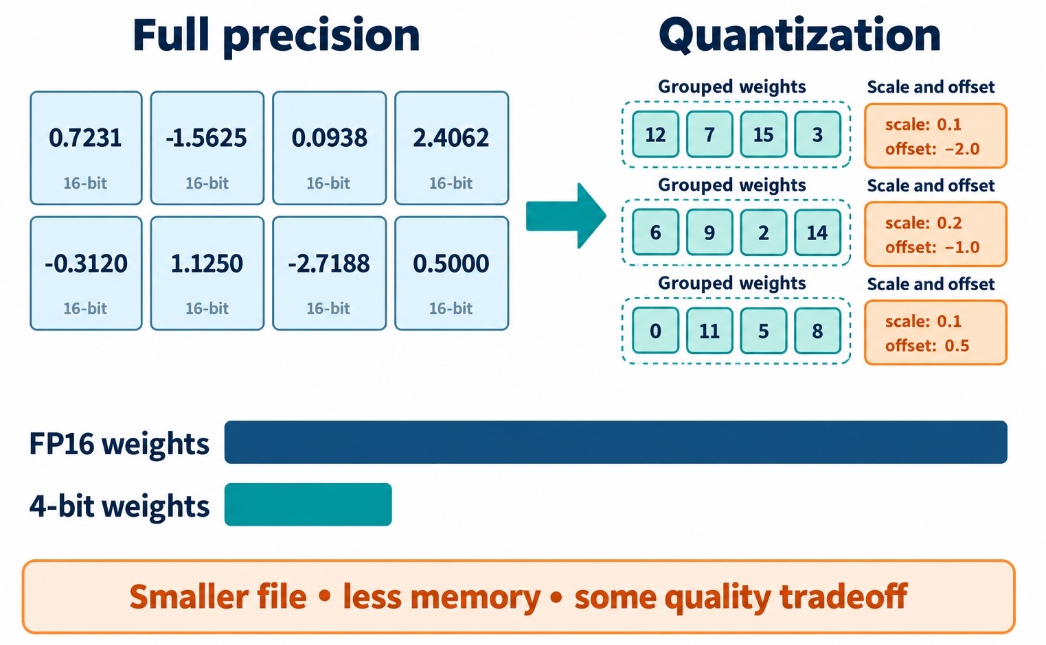
The second technique is the one you control directly, and it is the single most important concept for running models locally. Quantization is the process of storing each parameter using fewer bits, trading a little accuracy for a large reduction in memory and a nice boost in speed.

Recall that a parameter is just a number. In full precision, a model stores each one as a 16-bit floating-point value (fp16), which takes 2 bytes and can represent a wide range of values with fine gradations. Quantization replaces those with smaller integers. At 8 bits (int8), each weight is one byte, cutting memory in half. At 4 bits (int4), each weight is half a byte, cutting it in half again. A 4-bit model is roughly a quarter the size of the fp16 version.

The obvious question: how do you squeeze a wide-ranging floating-point number into a 4-bit integer that can only represent 16 distinct values, without destroying it? The answer is block-wise scaling. The weights are divided into small blocks (say, 32 weights per block). For each block, llama.cpp stores the low-bit integers plus a small amount of extra data: a scale (a multiplier) and sometimes a zero-point (an offset). To reconstruct an approximate original weight, you take the stored integer, multiply by the block’s scale, and add the offset. Because the scale is computed per block, it adapts to the local range of values, so a block of small weights and a block of large weights each get an appropriate multiplier. This is far more accurate than using one scale for the whole model.

Think of it like a shop rounding every price tag to the nearest whole dollar to make the labels smaller, while keeping one small correction note per aisle recording the average rounding error on that aisle. Each individual price loses a little precision, but because the correction is tracked per aisle rather than for the whole shop, the totals still come out very close to the originals. The low-bit integers are the rounded prices; the per-block scale is the per-aisle correction note.

That block-wise detail explains the otherwise baffling zoo of quantization names you see on Hugging Face. Here is a decoder for the ones you will actually encounter:

Name	Bits (approx)	What it means	When to reach for it
Q8_0	~8.5	8-bit, legacy block format, one scale per block	Highest practical quality, when memory is not tight
Q6_K	~6.6	6-bit, “K-quant” with smarter per-block scaling	Very close to 8-bit, noticeably smaller
Q5_K_M	~5.7	5-bit K-quant, Medium mix	A strong quality/size balance
Q4_K_M	~4.8	4-bit K-quant, Medium mix	The common default: best all-round tradeoff
Q4_K_S	~4.6	4-bit K-quant, Small mix	Slightly smaller than Q4_K_M, slightly lower quality
Q4_0	~4.5	4-bit, older legacy block format	Simple and fast, superseded by Q4_K_M for quality
IQ4_XS	~4.3	4-bit “i-quant”, extra-small	Smallest 4-bit, uses more CPU to decode

In the example above, the number is the bit width per weight, so lower means smaller and faster but less accurate. The K suffix marks the newer “K-quant” formats, which use a more sophisticated per-block scheme (mixing a couple of bit widths within the block and storing scales more cleverly) to get more quality out of the same bit budget than the older _0 formats. The S and M suffixes stand for Small and Medium, which describe how aggressively the format mixes in lower-precision pieces: Medium keeps a few important weight groups at higher precision for better quality, Small shaves those down for a smaller file. The IQ prefix marks “i-quants”, which use an even more advanced encoding to pack quality into very low bit counts, at the cost of being slower to decode on CPU. For a first model, the one to reach for is Q4_K_M: it is the widely-agreed sweet spot.

💡 You will not find every quant for every model. The auto-converted repositories from ggml-org on Hugging Face typically ship only Q4_0, Q8_0, and a full-precision BF16. The full K-quant and i-quant range usually comes from the official model publisher’s own GGUF repository or from prolific community packagers like bartowski and unsloth. If a repo does not list the quant you want, search Hugging Face for another repo of the same model that does.

The effect of quantization

So what do you actually gain and lose? The gains are concrete. Memory drops roughly in proportion to the bit width, so a 4-bit model is about a quarter the size of fp16. Speed improves too, because the biggest bottleneck in generation is moving weights from memory to the compute units, and smaller weights mean less data to move per token.

The loss is quality, and the standard way to measure it is perplexity: a number that captures how “surprised” the model is by real text, where lower is better and a well-behaved model stays close to its full-precision score. The important finding, repeated across many models, is that the quality loss is not linear. Going from fp16 to 8-bit is nearly free, barely measurable. Going to Q4_K_M costs a small, usually acceptable amount. Going below 4 bits is where quality starts to fall off a cliff, and the drop is worse for small models than large ones, because a tiny model has less redundancy to spare.

That last point is the practical lesson for laptop-scale models. For a 70B model, an aggressive 3-bit quant can still be excellent, because there is so much redundancy to trim. For a sub-1B model, the same aggressive quant can turn it incoherent. On a tiny model, stay at Q4_K_M or higher, and if you have the memory, Q8_0 costs you almost nothing in quality. The sweet spot for small local models sits squarely in the 4-bit-to-8-bit range.

---

How Local Models Run Fast

Shrinking the model gets it to fit. The next question is how it runs at a usable speed once it does. The answer is mostly one data structure, the KV cache, plus a few supporting tricks. This section is the mechanical heart of local inference, so we will take it slowly.

The KV cache in depth

Remember that attention, inside every transformer layer, looks back at every previous token to decide what is relevant right now. Here is the problem that creates. To generate token number 500, the model needs attention to compare the current position against all 499 tokens before it. The information attention needs from each previous token is two vectors per layer, historically called the key and the value (hence “K” and “V”). If the model recomputed those keys and values for all 499 previous tokens every single time it generated one new token, generation would get catastrophically slower as the text grew, because the work per token would scale with the length of everything so far.

The KV cache is the fix, and the idea is simple: compute each token’s keys and values once, then store them. When a token is first processed, each layer computes its key and value vectors and writes them into the cache. From then on, every future token’s attention step reads those stored vectors back instead of recomputing them. The only new work per generated token is computing the key and value for that one new token and reading the rest from the cache.

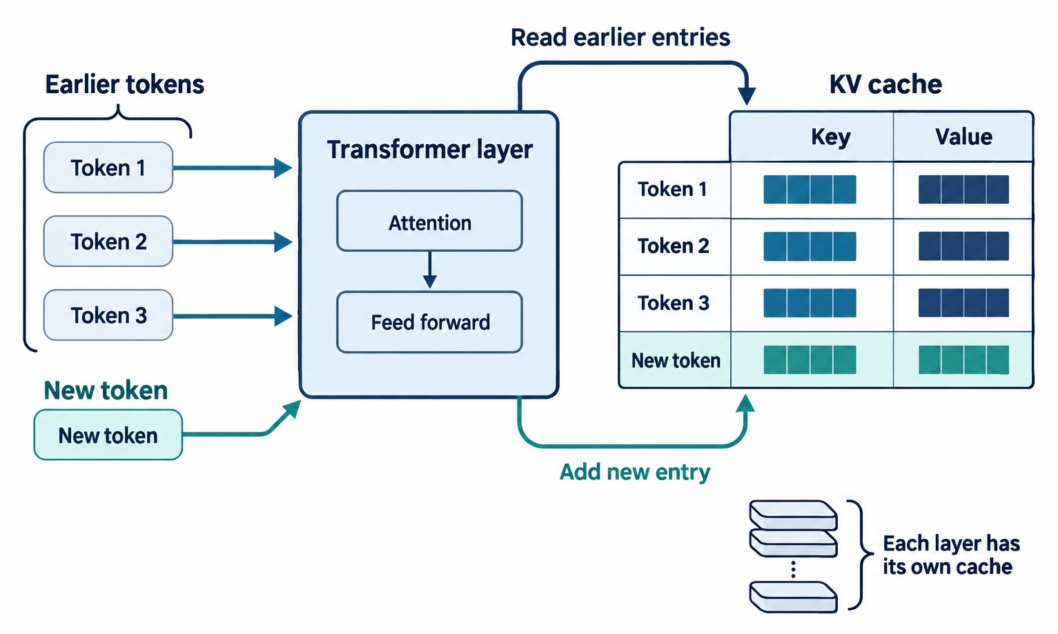
Think of it like taking notes in a long meeting. Without notes, every time someone makes a new point, you would have to mentally replay the entire meeting from the start to put it in context, which gets slower and slower as the meeting drags on. With notes, you glance back at what you have already written and just add the new point. The KV cache is the model’s notes: written once per token, read back cheaply forever after.

This also explains a cost that catches people out. The cache holds two vectors per token, per layer, for every token in the context. So its memory grows linearly with the length of the conversation and in proportion to the number of layers. A short prompt uses a little cache; a long conversation uses a lot. On a tiny model with a few dozen layers, a few thousand tokens of context is only a few hundred megabytes of cache, but on a large model with a long context it can rival the size of the weights themselves. The cache is why a model’s memory use is not fixed: it starts at the weight size and climbs as the context fills.

Prefill vs decode

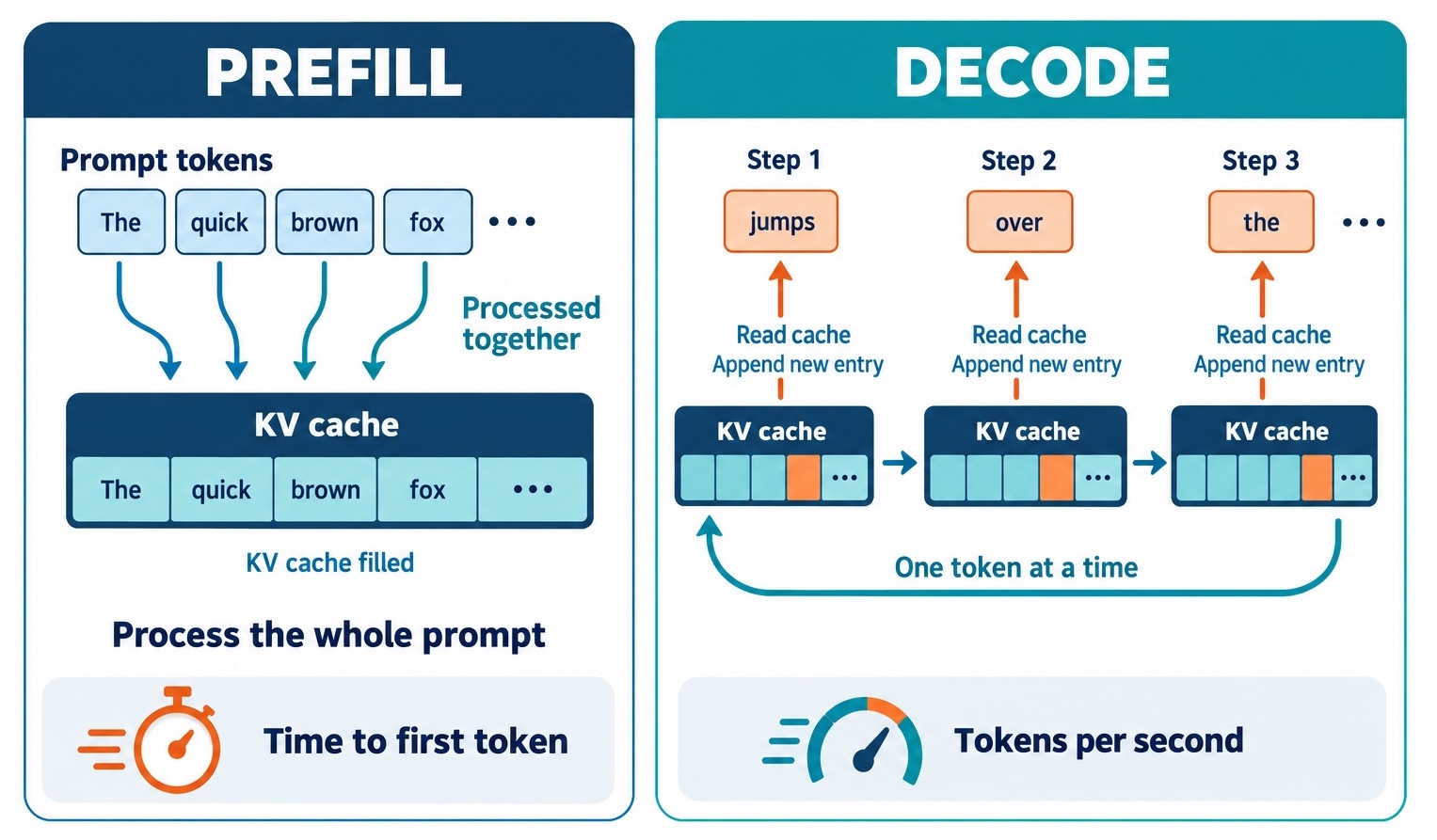
Generation happens in two distinct phases, and knowing the difference explains almost every “why is it slow right here?” question. The first phase is prefill: the model processes your entire prompt in one go. Because all the prompt tokens are already known, the model can compute their keys and values in parallel, in a single efficient pass, filling the KV cache for the whole prompt at once. The second phase is decode: the model generates the response one token at a time, each new token requiring its own pass that reads the whole cache and appends one new entry.

Think of it like cooking from a recipe. First you read the whole recipe end to end to take it all in at once, which is prefill: a single pass over everything already written. Then you cook it one step at a time, each step building on the ones before, which is decode: strictly sequential, one action after another.

Prefill (parallel, fills the cache):
  [The] [capital] [of] [France] [is]   -> all processed at once

Decode (one token at a time, reads the cache):
  ... -> [Paris]
  ... [Paris] -> [,]
  ... [Paris] [,] -> [a]

In the example above, prefill takes the five prompt tokens and processes them together in one parallel pass, computing and storing all their keys and values in the KV cache before any output appears. Decode then runs a loop: produce “Paris”, append it, produce ”,”, append it, and so on, each step a separate pass through the full model that reads the entire cache and writes one new entry. This is why a very long prompt feels slow before any text shows up: that delay is prefill chewing through the whole prompt. Once decode starts, tokens stream out at a steadier pace. The two phases give us two different speed numbers that matter: time to first token (dominated by prefill, so it grows with prompt length) and throughput in tokens per second (dominated by decode, so it reflects how fast the model generates once it gets going). A model can have a quick time to first token but slow throughput, or the reverse, and llama-bench reports both separately for exactly this reason.

KV cache quantization

Here is a nice trick that follows directly from the two ideas above. If the KV cache is just more numbers in memory, and quantization shrinks numbers, then you can quantize the cache too. By default the cache is stored in 16-bit precision, but llama.cpp lets you store the keys and values at lower precision with the --cache-type-k and --cache-type-v flags, for example setting both to q8_0. This roughly halves the cache’s memory footprint, which directly lets you fit a longer context (more tokens) in the same amount of memory.

# Store the KV cache in 8-bit instead of the default 16-bit
llama-cli -hf ggml-org/Qwen3.5-0.8B-GGUF:Q8_0 -fa on --cache-type-k q8_0 --cache-type-v q8_0 -c 8192

In the example above, --cache-type-k q8_0 and --cache-type-v q8_0 tell llama.cpp to store the key and value vectors as 8-bit values rather than 16-bit, cutting the cache size roughly in half and freeing memory to raise -c (the context length) to 8192 tokens. The -fa on is not optional window dressing here: cache quantization requires flash attention, an optimized attention implementation enabled with -fa, because the quantized-cache code path is implemented inside it. Without -fa turned on, the cache-type flags are ignored or rejected. The tradeoff is the same as any quantization: an 8-bit cache is nearly lossless, while pushing the cache down to 4-bit saves more memory but can measurably degrade output quality, more so on small models. Reach for an 8-bit cache first; go lower only if you are desperate for context length and have tested that the quality still holds.

💡 Flash attention is worth enabling in general, not just for cache quantization. It computes attention in a more memory-efficient way that avoids materializing a large intermediate matrix, which both saves memory and speeds things up, especially at longer contexts. On recent builds -fa accepts on, off, or auto; on older builds it was a bare on/off switch. If a flag form is rejected, check llama-cli --help against your build.

Other speed optimizations

A few more mechanisms round out the picture. mmap is how llama.cpp loads weights by default: instead of reading the whole file into memory up front, it memory-maps the file, letting the operating system page in parts of it on demand. This makes startup nearly instant and lets multiple processes share the same weights in memory. Continuous batching is a server-side feature where llama-server interleaves tokens from multiple simultaneous requests to keep the hardware busy, so throughput stays high when several clients are connected. The -ngl flag (number of GPU layers) controls how many of the model’s layers are offloaded to the GPU; on an M2 Pro with enough memory you offload all of them. Context size, set with -c, is a direct tradeoff: a larger context lets the model remember more but costs more KV cache memory and makes prefill slower.

Finally, one paragraph on speculative decoding, because you will see it mentioned. It is a technique where a tiny, fast “draft” model proposes several tokens ahead, and the main model verifies them in a single batched pass, accepting the ones it agrees with. When the draft is often right, this generates multiple tokens for roughly the cost of one, speeding up decode. It adds complexity (you run two models) and helps most on larger models, so it is more of an advanced tuning option than something you need on day one. The llama.cpp documentation covers it if you want to experiment.

---

GGUF, Model Formats, and Hugging Face

We keep mentioning GGUF. It is time to pin down exactly what it is, how it differs from the other formats you will trip over, and how you actually get these files onto your machine. Why does llama.cpp use its own format at all instead of just reading whatever the model publisher uploaded?

What GGUF is

GGUF (GGML Universal Format) is the single-file container format that llama.cpp reads. One .gguf file holds everything needed to run the model: the quantized tensors (the actual weights, in whatever quant you chose), plus a block of metadata, plus the tokenizer, plus the chat template, plus a record of which quantization type was used. It is deliberately designed to be memory-mapped, which ties back to the mmap loading we just discussed: the layout on disk matches the layout in memory, so the OS can map the file directly without parsing and reshuffling it first.

That “everything in one file” property is the whole point. In the example of running a model, you do not assemble a config file, a separate tokenizer file, and a weights file and hope their versions match. You point llama.cpp at one .gguf and it has the weights to run, the tokenizer to turn your text into tokens, and the chat template to format your messages correctly, all guaranteed to belong together because they were packaged together. The metadata inside also records things like the model’s architecture and its trained context length, so llama.cpp knows how to set itself up just from reading the file header.

Other formats and how they differ

GGUF is not the only format, and knowing the others clarifies why GGUF exists. safetensors is the standard format on Hugging Face for full-precision weights. It is a safe, fast container for tensors (the “safe” refers to it not executing arbitrary code on load, unlike the format it replaced), but it holds only the raw weights, usually in fp16 or bf16, with no built-in quantization, tokenizer, or chat template. It is what you convert from. PyTorch .bin files are the older default, based on Python’s pickle serialization, which can execute code when loaded and is the unsafe format safetensors was created to replace. GGML was llama.cpp’s own earlier format, now fully superseded by GGUF, which fixed GGML’s lack of extensible metadata. MLX is Apple’s framework and format for running models natively on Apple Silicon, a genuine alternative to llama.cpp on a Mac. GPTQ and AWQ are GPU-oriented quantization formats designed for datacenter inference stacks rather than CPU-and-Metal local use.

So why GGUF for llama.cpp? Because llama.cpp targets running quantized models efficiently on everyday hardware, including CPUs and Apple Silicon, and it needs a format that bundles the quantized weights with the tokenizer and template and maps straight into memory. The full-precision safetensors format was never meant for that, and the GPU-datacenter formats target different hardware. GGUF is the format built for exactly llama.cpp’s job.

Hugging Face

Hugging Face is the hub where almost all of these models live. Think of it like a package registry (npm, but for models): organizations and individuals publish model repositories, and you pull from them. A single model usually has multiple repositories: the original publisher’s full-precision safetensors repo, and one or more GGUF repos (from the publisher, from ggml-org, or from community packagers) that contain the quantized .gguf files. Inside a GGUF repo, each quantization is a separate file, named with the quant it contains, like Qwen3.5-0.8B-Q8_0.gguf.

The convenient part is that llama.cpp can pull directly from Hugging Face. The -hf flag takes an org/repo identifier and downloads the GGUF for you, caching it locally so the next run is instant.

# Download (first run) and run a specific quant directly from Hugging Face
llama-cli -hf ggml-org/Qwen3.5-0.8B-GGUF:Q8_0 -p "Explain what a tokenizer does, in two sentences." -n 128

In the example above, -hf ggml-org/Qwen3.5-0.8B-GGUF names the Hugging Face repository, and the :Q8_0 suffix selects which quantization file to download from it, so you are not forced to copy the exact filename. llama.cpp resolves the repo, downloads the matching .gguf into its local cache on the first run, and reuses the cached copy afterward. If you omit the :quant suffix it picks a default. This caching is why running a model is effectively a one-liner: the first run pulls the file, and every run after reuses the cached copy, so only that first invocation needs the network.

💡 You can also roll your own GGUF from a full-precision model. llama.cpp ships convert_hf_to_gguf.py, which converts a safetensors model into an fp16 GGUF, and llama-quantize, which turns that fp16 GGUF into any quant you want (llama-quantize model-f16.gguf model-Q4_K_M.gguf Q4_K_M). This is how the GGUF repos on Hugging Face are produced in the first place, and it is useful when a model you want has no GGUF repo yet, or when you want a specific quant nobody has published.

---

Setting Up llama.cpp on an Apple M2 Pro

Enough theory. Let’s get llama.cpp onto an actual machine and confirm it is using the GPU. Everything here assumes an Apple M2 Pro with Apple Silicon and the Metal backend, but the Homebrew path works on any modern Mac.

Installing

The simplest install is Homebrew.

# Install the prebuilt llama.cpp package
brew install llama.cpp

In the example above, Homebrew downloads a prebuilt llama.cpp with Metal support already compiled in and puts the llama-cli, llama-server, and llama-bench programs on your path. On Apple Silicon, the Metal GPU backend is enabled by default, so there is nothing extra to turn on: a freshly installed llama.cpp will use the GPU out of the box. If you would rather build from source (to get the very latest commit, or to tune build options), you clone the repository and build it with CMake, and on a Mac the Metal backend is included automatically unless you explicitly disable it. The source route is documented in the project’s build guide.

You confirm Metal is active by looking at the startup logs, which we will read in detail in the next section. The short version: when you run any model, llama.cpp prints lines mentioning Metal and the number of layers offloaded to the GPU. If you see those, the GPU is in use.

The binaries you will use

Three programs cover everything in this article. llama-cli runs a model for a single prompt or an interactive chat, and it is where you will experiment. llama-server starts a long-lived process exposing an HTTP API, which is how you serve a model to other programs. llama-bench runs a model under controlled conditions and reports its speed, which is how you measure the effect of a quant or a cache setting. There are more programs in a full install (for quantizing, for perplexity measurement, and so on), but these three are the core.

💡 llama.cpp moves fast. Flags get renamed, defaults shift between releases, and the project has been consolidating its command-line programs over time, so the exact invocation on your build may differ slightly from any article, including this one. Before trusting a flag, run llama-cli --help (or --help on whichever program) and check it against your installed version. Treat the flag names here as correct-at-time-of-writing, not eternal.

Picking and downloading the model

For a first model, use the one the llama.cpp quick-start itself reaches for: ggml-org/Qwen3.5-0.8B-GGUF, a sub-1B instruct model from the Qwen family. It is small, recent, and good enough to be genuinely useful, which makes it ideal for learning. That repository ships three files: a full-precision BF16, a 4-bit Q4_0, and an 8-bit Q8_0.

# Download the 8-bit quant (highest quality in this repo)
llama-cli -hf ggml-org/Qwen3.5-0.8B-GGUF:Q8_0 -p "Say hello in three languages." -n 64

# Download the 4-bit quant (smaller and faster)
llama-cli -hf ggml-org/Qwen3.5-0.8B-GGUF:Q4_0 -p "Say hello in three languages." -n 64

In the example above, the two commands pull different quantizations of the same model: Q8_0 is about 830 MB and the closest thing to the original model’s quality, while Q4_0 is about 560 MB, smaller and quicker to run but with a bit more quality loss. On a model this tiny the Q8_0 is cheap enough that it is the sensible default; the Q4_0 matters more when you move to larger models where the size difference is measured in gigabytes. If you specifically want the Q4_K_M quant discussed earlier (the usual all-round sweet spot), this auto-converted repo does not include it, so pull it from a community repo such as bartowski or unsloth that packages the full K-quant range for Qwen models.

When a sub-1B model is not capable enough, the natural next step up is the roughly 1.7B sibling, ggml-org/Qwen3-1.7B-GGUF. It needs more memory and runs slower, but it reasons noticeably better. The same download pattern applies, just with the larger repo name. Like the 0.8B anchor, this is an auto-converted repo that ships only Q4_0, Q8_0, and BF16, so if you want the Q4_K_M quant recommended later, pull the 1.7B from a bartowski or unsloth repo that packages the full K-quant range instead.

Will it fit? The memory math

Before downloading something large, you want to answer one question: will this fit in my memory? Here is a formula concrete enough to actually use. Total memory is roughly the weights plus the KV cache plus a fixed overhead:

weights    ≈ parameters × (bits_per_weight / 8)
kv_cache   ≈ 2 × n_layers × context × kv_dim × bytes_per_element
total      ≈ weights + kv_cache + ~0.5–1 GB overhead

In the example above, the weights term is just the parameter count times the bytes each weight takes, so a 0.8B model at 8 bits (one byte each) is about 0.8 GB, and at 4 bits about 0.4 GB. The KV cache term is the one people forget: the 2 is for storing both keys and values, n_layers is the model’s layer count, context is how many tokens you set with -c, kv_dim is the per-layer size of each key/value vector (which depends on the model’s architecture), and bytes_per_element is 2 for the default 16-bit cache or 1 for an 8-bit cache. The overhead is compute buffers and the like. The practical takeaway: for a sub-1B model with a few thousand tokens of context, the weights dominate and the cache is a few hundred megabytes, so the whole thing lands comfortably under 2 GB and runs with room to spare in a 16 GB M2 Pro. Worked the other way, a 7B model at Q4_K_M is about 4 GB of weights plus a cache that grows with context, which still fits in 16 GB but leaves far less headroom for a long context or other applications.

💡 On Apple Silicon the GPU draws from the same unified memory pool as everything else, so “will it fit in my 16 GB” really means the model plus its cache plus macOS plus your browser plus everything else. Leave several gigabytes of headroom. If a model loads but your whole machine starts swapping and crawling, you are over the real budget even though the model technically fit.

---

Running Your First Model from the CLI

With llama.cpp installed and a model chosen, let’s actually run it and understand every part of what happens. The CLI is where you build intuition before writing any code.

A one-line run

Here is a complete, real invocation with the flags spelled out.

# Run a single prompt, generating up to 256 tokens, with an 8192-token context, all layers on the GPU
llama-cli -hf ggml-org/Qwen3.5-0.8B-GGUF:Q8_0 -p "Give me three ideas for naming a pet turtle." -n 256 -c 8192 -ngl 99

In the example above, each flag maps to a concept we have already built up. -hf ggml-org/Qwen3.5-0.8B-GGUF:Q8_0 names the Hugging Face repo and quant to download and run. -p is the prompt text. -n 256 caps generation at 256 tokens, so the model stops there even if it would keep going (the decode loop runs at most this many times). -c 8192 sets the context window to 8192 tokens, which sizes the KV cache and determines how much text the model can consider at once. -ngl 99 offloads up to 99 layers to the GPU; since this model has far fewer than 99 layers, the effect is “put all of them on the GPU”, which is what you want on an M2 Pro. Set -ngl 0 and the model runs entirely on the CPU, which is a useful comparison to feel how much Metal is doing for you.

Reading the startup logs

Before any generated text appears, llama.cpp prints a wall of log lines. Most of it is diagnostic, but a few lines tell you whether things are set up correctly.

load_tensors: offloaded 29/29 layers to GPU
load_tensors:      Metal buffer size =   810.00 MiB
llama_context: n_ctx = 8192
llama_kv_cache: Metal KV buffer size = 112.00 MiB

In the example above, offloaded 29/29 layers to GPU is the line you want to see: every layer is on the GPU, so decode will run at full Metal speed. If it said 0/29, the GPU is not being used and you forgot or mis-set -ngl. The Metal buffer size line shows the weights occupying GPU-accessible memory, matching the file size as expected. The n_ctx = 8192 confirms the context you requested was accepted (if you ask for more than the model was trained to handle, llama.cpp caps you at or warns about the trained maximum, and the log shows the real value). The KV buffer size line is the KV cache we have been discussing, sized here for 8192 tokens; raise -c and this number grows, lower it and it shrinks. Reading these four lines tells you the GPU is engaged, how much memory the weights and cache take, and that your context setting took effect.

Turning on flash attention and cache quantization

Now layer in the KV cache optimizations from earlier and watch the numbers move.

# Same run, but with flash attention and an 8-bit KV cache
llama-cli -hf ggml-org/Qwen3.5-0.8B-GGUF:Q8_0 -p "Give me three ideas for naming a pet turtle." -n 256 -c 8192 -ngl 99 -fa on --cache-type-k q8_0 --cache-type-v q8_0

In the example above, adding -fa on enables flash attention, and --cache-type-k q8_0 with --cache-type-v q8_0 stores the cache in 8-bit. The measurable change shows up in the startup logs: the KV buffer size line drops to roughly half of what it was with the default 16-bit cache, because each cached key and value now takes one byte instead of two. On a tiny model with a short context that saving is small in absolute terms, but the same flags on a larger model or a much longer context free up gigabytes, which is often the difference between fitting a long conversation and running out of memory. Flash attention also tends to improve speed at longer contexts, which the next tool lets us actually measure.

Benchmarking with llama-bench

How do you know a quant or cache setting actually helped, rather than just feeling faster? You measure it. llama-bench runs the model under controlled conditions and reports speed through exactly the prefill-vs-decode lens we built earlier.

# Benchmark prompt-processing (prefill) and generation (decode) speed
llama-bench -m ~/Library/Caches/llama.cpp/ggml-org_Qwen3.5-0.8B-GGUF_Qwen3.5-0.8B-Q8_0.gguf -p 512 -n 128

In the example above, -m points at a local GGUF file (the path is where -hf cached the download; your exact path may differ, so check the cache directory). The -p 512 tells llama-bench to measure processing a 512-token prompt, which is the prefill phase, and -n 128 tells it to measure generating 128 tokens, which is the decode phase. The output is a table with two key rows: a pp512 number (prompt processing, in tokens per second) and a tg128 number (text generation, in tokens per second). Prompt processing is typically much faster per token than generation, because prefill runs in parallel while decode is strictly one token at a time. These two numbers map directly onto the user-visible experience: pp governs how long you wait before the first token appears (time to first token), and tg governs how fast the response then streams. Run the benchmark with Q8_0 versus Q4_0, or with and without the 8-bit cache, and you can see precisely how each setting moves prefill speed, decode speed, and memory, instead of guessing.

---

Getting Good Output: Templates, Sampling, and Context

You can now run a model and measure it. But if you ran that earlier -p "..." command and got rambling, repetitive, or oddly-formatted output, you hit the single biggest source of confusion with local models. It is almost never the model being dumb. It is one of three things: the chat template, the sampling settings, or the context window. Let’s fix all three.

Chat templates

An instruct model was trained on conversations wrapped in a very specific format, with special tokens marking where each speaker’s turn begins and ends. That format is the chat template. Recent Qwen models use a format called ChatML, where each message is wrapped like <|im_start|>user … <|im_end|>, with <|im_start|> and <|im_end|> being the special tokens we met back in the tokenization section. The model learned that an assistant reply comes right after an <|im_start|>assistant marker, so that structure is the cue that tells it to answer rather than continue your text. Think of it like the fixed To, From, and Subject header on an envelope: the model was trained to only “open the letter” and respond when the message arrives in that exact envelope format, and plain text with no envelope leaves it unsure whether to reply at all.

Here is the problem with a raw -p prompt. When you pass -p "What is a tokenizer?" with no template, the model receives those exact words with none of the ChatML scaffolding it was trained to expect. It has no <|im_start|>assistant cue telling it “your turn to answer now”, so it falls back on raw continuation and often produces rambling garbage: more questions, a fake dialogue, or a wandering monologue. The fix is to apply the chat template, and the good news is that the template is embedded in the GGUF file (remember, the format bundles it), so llama.cpp knows the right one automatically. You just have to tell it to use conversation mode.

# Conversation mode applies the model's embedded chat template automatically
llama-cli -hf ggml-org/Qwen3.5-0.8B-GGUF:Q8_0 -cnv

In the example above, -cnv puts llama-cli into conversation mode: it reads the chat template out of the GGUF, wraps whatever you type in the correct ChatML markers, adds the <|im_start|>assistant cue, and drops you into an interactive back-and-forth where each of your messages is formatted correctly before it reaches the model. This is why the same model that produced garbage from a raw -p prompt suddenly answers cleanly in -cnv mode: nothing about the model changed, only whether its input was formatted the way it was trained to expect. The same split exists in the server, which we will see later: its /v1/chat/completions endpoint applies the template for you, while the lower-level /completion endpoint does not and expects you to format the prompt yourself.

💡 If a local model is producing bizarre output, suspect the chat template before you blame the model or the quant. Running through -cnv or the chat-completions endpoint fixes the large majority of “this model seems broken” reports. Raw completion mode has its uses, but only when you are deliberately formatting the prompt yourself.

Sampling parameters

Once the prompt is formatted correctly, the model produces a probability distribution over the next token, and sampling is how one token gets chosen from that distribution. The settings here control the personality of the output: how creative, how focused, how repetitive. Each is a dial worth understanding.

temperature scales how much the model favors high-probability tokens. At a low temperature (near 0) it almost always picks the single most likely token, giving focused, deterministic, sometimes repetitive output. At a high temperature (above 1) it flattens the distribution, picking less likely tokens more often, giving creative, varied, sometimes incoherent output. top-k restricts the choice to only the k most likely tokens, discarding the long tail of unlikely ones. top-p (also called nucleus sampling) instead keeps the smallest set of top tokens whose probabilities add up to p, so it adapts the cutoff to the distribution’s shape. min-p keeps only tokens above a fraction of the top token’s probability, another adaptive cutoff that works well with higher temperatures. repeat-penalty reduces the probability of tokens that recently appeared, which combats the loops tiny models love to fall into. seed fixes the random number generator so the same inputs produce the same output, which is essential when you want reproducible results.

# Deterministic, focused output: low temperature and a fixed seed
llama-cli -hf ggml-org/Qwen3.5-0.8B-GGUF:Q8_0 -cnv --temp 0.2 --top-p 0.9 --top-k 40 --repeat-penalty 1.1 --seed 42

In the example above, --temp 0.2 keeps the output focused and factual by strongly favoring the most likely tokens, which is what you want for a question with a correct answer. --top-p 0.9 and --top-k 40 cap how far down the probability list the model is allowed to reach, trimming the unlikely tail so it does not occasionally pick something bizarre. --repeat-penalty 1.1 gently discourages the model from repeating recent tokens, which matters more on small models that are prone to getting stuck in loops. --seed 42 fixes the randomness, so rerunning this exact command gives the exact same answer, which is invaluable for debugging and for comparing two settings fairly. For creative tasks you would raise the temperature and loosen top-p; the point is that these dials, not the model, often decide whether output feels sharp or sloppy.

The context window

The context window is the maximum number of tokens the model can consider at once: your prompt, the conversation history, and the response it is generating, all counted together. You set it with -c, but with a hard ceiling: it cannot exceed the length the model was trained for, which is recorded in the GGUF metadata. llama.cpp honors -c up to that trained length and caps you at (or warns you about exceeding) the trained maximum beyond it, since going further needs a trick called RoPE scaling (stretching the model’s positional encoding so it can address token positions it never saw during training, at some cost to quality) rather than being free. This window is not a soft preference. It is a wall.

What happens when a conversation grows past the window? The model cannot simply remember more, so llama.cpp has to drop something, and what it drops is the oldest tokens: this is context truncation.

By default, llama-server does not stop when you hit the ceiling. It performs a context shift. It keeps a protected region at the very front, the n_keep tokens, which is normally your system prompt, then discards a chunk of the oldest conversation tokens after it and renumbers the surviving tokens so their positions stay contiguous. Internally this means part of the KV cache is thrown away and the remaining entries are shifted down, which costs a small burst of recompute right at that moment. The practical upshot is specific and worth internalizing: the middle of a long chat evaporates first while a pinned system prompt survives, so the model keeps obeying its instructions but forgets what you told it twenty messages ago. Context shift can also be turned off, and some flash-attention and cache-quantization combinations disable it automatically, in which case generation simply halts when the window fills instead of sliding forward. Knowing which of the two behaviors your build does turns “why did it suddenly stop?” or “why did it forget?” into something you can predict rather than a mystery.

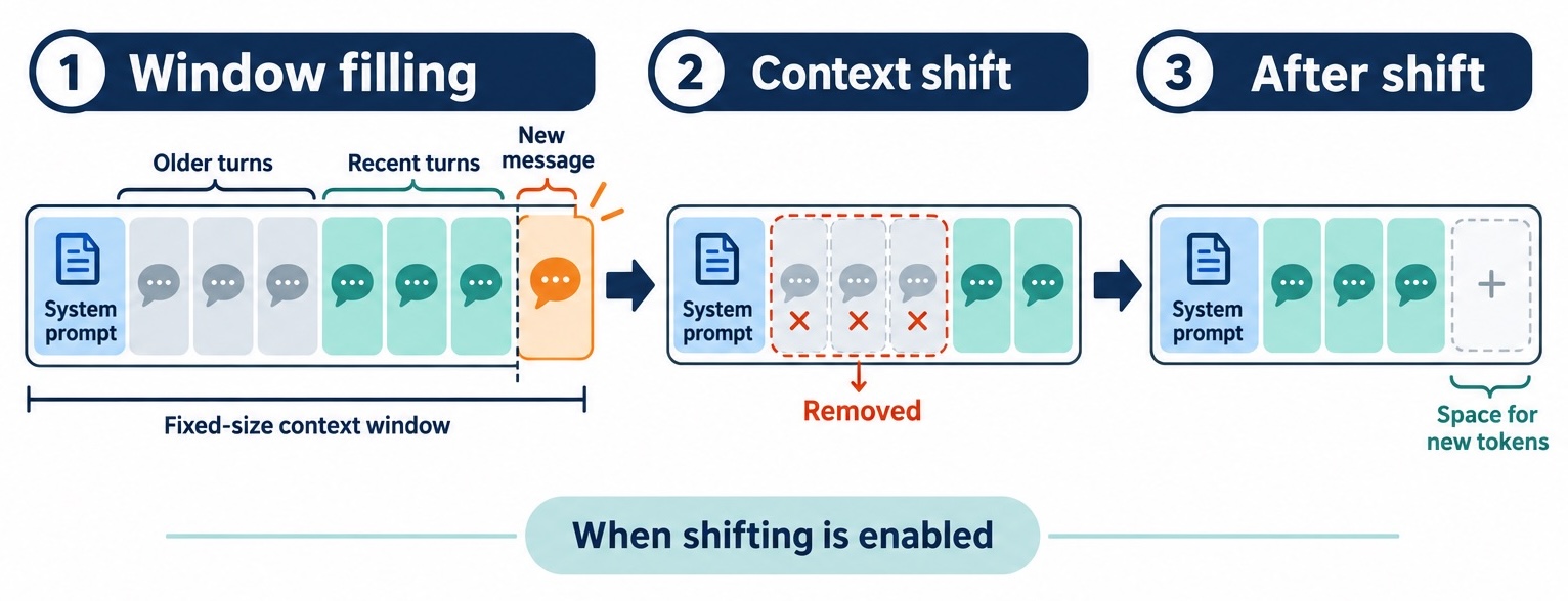
This is the signature pain point of tiny local models, and it deserves a concrete walk-through because it feels like a bug the first time you hit it. Suppose you are using a small model with a modest context and you have a long back-and-forth:

[earlier] You: My name is Dana and I'm planning a trip to Lisbon.
[earlier] Model: Great! Lisbon is wonderful. What would you like to know?
... 40 more messages about restaurants, neighborhoods, and day trips ...
[now]     You: Remind me, what was my name again?
[now]     Model: I'm sorry, I don't have that information.

In the example above, the model is not being obtuse. The first exchange, where you said your name was Dana, scrolled out of the context window dozens of messages ago. Those tokens were truncated to make room for the newer ones, so by the time you ask, the sentence containing “Dana” is simply not in the model’s input anymore. It genuinely cannot see it. This is why small local models feel forgetful: a small context fills quickly, and once it does, the beginning of your conversation silently evaporates. The practical defenses are to raise -c if the model’s trained maximum and your memory allow, to keep conversations focused, and to re-state crucial facts periodically rather than assuming the model still has them. Understanding that truncation is happening, and why, turns a baffling behavior into a predictable one you can design around.

Thinking mode

One more recent wrinkle. Models in the recent Qwen generation can emit a thinking block: a stretch of output wrapped in <think> and </think> tags where the model reasons step by step before giving its final answer. The idea is that letting the model “work out loud” improves its answers on problems that need multi-step reasoning, like math or logic puzzles. The content inside the tags is the model’s scratch work; the real answer comes after the closing tag.

Thinking helps on genuinely hard problems and is pure overhead on simple ones, where it just burns tokens and time restating the obvious before answering. On a tiny model with limited context, that overhead also eats into your window. You can turn it off: recent Qwen models respond to a /no_think instruction in the prompt, and llama.cpp exposes --chat-template-kwargs '{"enable_thinking": false}' (recent builds also accept --reasoning-budget 0), which flips the exact switch the Qwen chat template reads to decide whether to emit a thinking block. If a model is spending ten seconds “thinking” before telling you the capital of France, switching thinking off is the fix. Reach for it when the task genuinely benefits from reasoning, and turn it off for quick factual or formatting tasks where it only adds latency.

💡 When thinking is on, the <think>...</think> block is part of the generated output by default, not a separate piece of metadata. So if you naively concatenate tokens or read message.content, the model’s scratch work ends up mixed into the answer you show the user, and worse, into anything you hand to JSON.parse. On the server, either strip everything up to and including </think> before using the result, or read the separate reasoning_content field that recent chat-completions builds expose, which carries the thinking apart from the final answer.

---

From CLI to Code

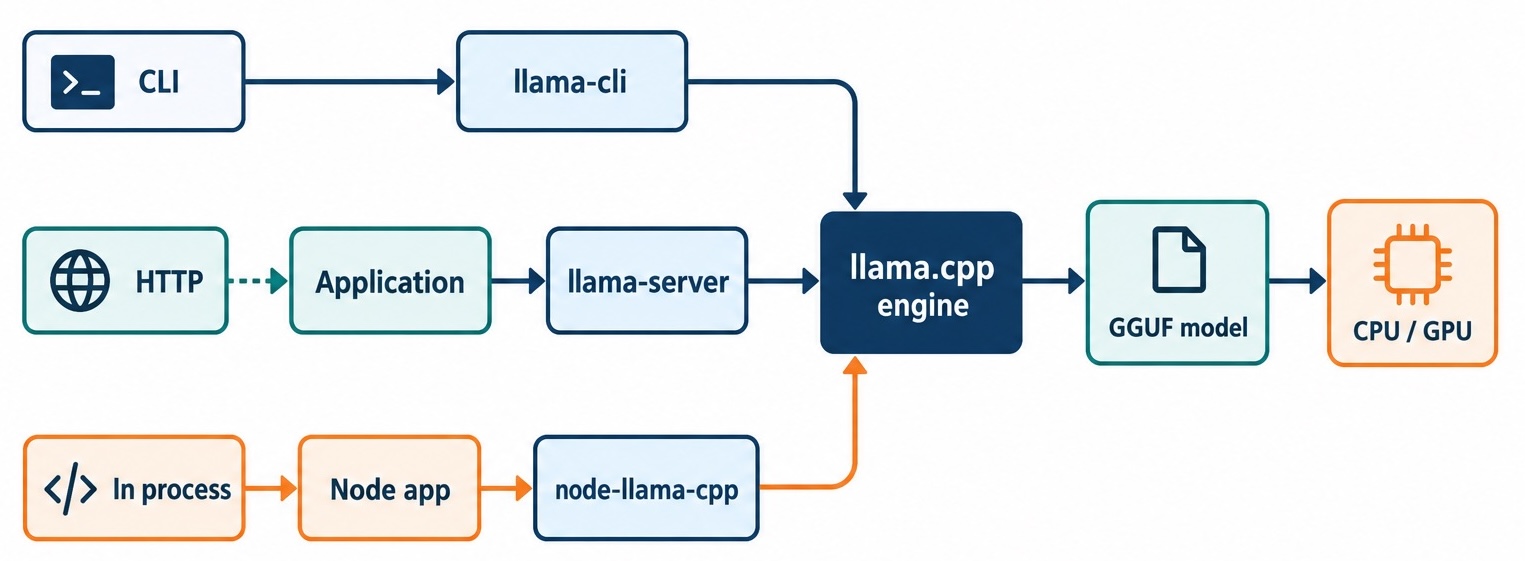
The CLI is for experimenting. Real applications need the model reachable from code. This is where people get confused about the shape of things: is the model a server I call, a library I import, or a subprocess I spawn? The honest answer is “any of the three”, and which one you pick depends on your situation. Let’s lay out how the pieces fit, then build each path in TypeScript.

How the pieces fit

There are three ways to run a model from code, and they differ in where the model lives relative to your application. The CLI (llama-cli) is an in-process one-off: a program that loads the model, does its work, and exits, which is perfect for experimenting but not for serving. The server (llama-server) is a long-lived process that loads the model once and exposes an HTTP API, so your application talks to it over the network (even if that network is just localhost). Bindings load the model inside your own application’s process, so there is no separate server and no HTTP at all; the model is a library you call directly.

Think of it like a database. You can run a one-off query from a CLI tool, you can run a database server your app connects to over a socket, or you can embed an in-process database like SQLite directly inside your app. Same data, three deployment shapes, chosen by your needs. The KV cache, worth noting, exists in all three, because it belongs to the inference context, not to any particular way of invoking it. Whether you go through the CLI, the server, or a binding, the model still builds and reads a KV cache exactly as described earlier.

Running llama-server

The server is the most common way to use a local model from an application, because it decouples the model (loaded once, kept warm) from your code (which can restart freely without reloading gigabytes of weights). You start it much like the CLI, and the performance flags carry over unchanged.

# Start an OpenAI-compatible server on port 8080, all layers on GPU, 8-bit KV cache
llama-server -hf ggml-org/Qwen3.5-0.8B-GGUF:Q8_0 -c 8192 -ngl 99 -fa on --cache-type-k q8_0 --cache-type-v q8_0 --port 8080 --parallel 4

In the example above, the model, context, GPU-offload, flash-attention, and cache-type flags are exactly the ones we used with llama-cli, because they configure the inference engine, which is the same underneath both programs. The new flags are server-specific: --port 8080 sets the HTTP port, and --parallel 4 creates four slots so the server can handle four requests at once, which is where the continuous batching mentioned earlier kicks in to keep the GPU busy across concurrent clients. Once it is running, the server exposes an OpenAI-compatible API, meaning its /v1/chat/completions endpoint speaks the same request and response shape as OpenAI’s, so any client written for OpenAI works against your local server with just a changed base URL.

Calling it from a TypeScript client

Because the server is OpenAI-compatible, calling it from TypeScript is a plain HTTP request to /v1/chat/completions.

// file: src/llm/client.ts
// A minimal client that sends a chat request to the local llama-server.
async function ask(question: string): Promise<string> {
  const response = await fetch("http://localhost:8080/v1/chat/completions", {
    method: "POST",
    headers: { "Content-Type": "application/json" },
    body: JSON.stringify({
      messages: [
        { role: "system", content: "You are a concise, helpful assistant." },
        { role: "user", content: question },
      ],
      temperature: 0.3,
      max_tokens: 256,
    }),
  });

  const data = await response.json();
  return data.choices[0].message.content;
}

In the example above, the request body is the OpenAI chat shape, and each field maps to a concept we have already covered. messages is the conversation as an array of role-tagged turns; the server runs these through the model’s embedded chat template (the ChatML formatting from the templates section) so you never assemble <|im_start|> markers by hand. The system message sets behavior, the user message is the question. temperature is the same sampling dial as the CLI’s --temp, controlling focus versus creativity. max_tokens caps the response length, exactly like -n, bounding the decode loop. The response comes back as choices[0].message.content, which is the generated text. This is the entire integration: a POST to localhost, parse the JSON, read the content. If you prefer, the official OpenAI SDK works against the same endpoint by setting its baseURL to http://localhost:8080/v1.

To stream tokens as they are generated rather than waiting for the whole response, you add stream: true and read the response as a stream of server-sent events.

// file: src/llm/stream.ts
// Stream tokens from the local server as they are generated.
async function askStreaming(question: string, onToken: (t: string) => void) {
  const response = await fetch("http://localhost:8080/v1/chat/completions", {
    method: "POST",
    headers: { "Content-Type": "application/json" },
    body: JSON.stringify({
      messages: [{ role: "user", content: question }],
      stream: true,
    }),
  });

  const reader = response.body!.getReader();
  const decoder = new TextDecoder();

  while (true) {
    const { value, done } = await reader.read();
    if (done) break;

    for (const line of decoder.decode(value).split("\n")) {
      if (!line.startsWith("data: ") || line.includes("[DONE]")) continue;
      const token = JSON.parse(line.slice(6)).choices[0].delta.content;
      if (token) onToken(token);
    }
  }
}

In the example above, stream: true tells the server to send the response incrementally instead of all at once. The server emits server-sent events, a simple format where each chunk arrives as a line beginning with data: followed by a JSON object. The code reads the response body as a stream, splits each arriving piece into lines, skips the keep-alive and the terminating [DONE] marker, and for each real data line pulls the new piece of text out of choices[0].delta.content (note delta, not message: streaming responses carry incremental deltas rather than a complete message). Each token is handed to the onToken callback the moment it arrives, which is what lets you render text appearing word by word. This streaming shape is why local models feel responsive: the first token can render in milliseconds, long before the full answer is done.

Integrating into your own HTTP server

The realistic production pattern is not calling llama-server directly from a browser. It is putting your own server in front of it, so you control authentication, rate limiting, logging, and prompt construction, while llama-server does only inference. Here is a minimal Express endpoint that forwards to it.

// file: src/server.ts
// An Express endpoint that forwards chat requests to a local llama-server.
import express from "express";

const app = express();
app.use(express.json());

const LLAMA_URL = "http://localhost:8080/v1/chat/completions";

app.post("/api/chat", async (req, res) => {
  const llamaResponse = await fetch(LLAMA_URL, {
    method: "POST",
    headers: { "Content-Type": "application/json" },
    body: JSON.stringify({
      messages: [
        { role: "system", content: "You are a support assistant for Acme." },
        { role: "user", content: req.body.message },
      ],
      max_tokens: 512,
    }),
  });

  const data = await llamaResponse.json();
  res.json({ reply: data.choices[0].message.content });
});

app.listen(3000);

In the example above, your Express server owns the system prompt and the request shape, so the browser only ever sends a raw user message and never gets to set the system instruction or the token limit, which is exactly the control you want in production. The endpoint forwards to LLAMA_URL on localhost, where llama-server is running as a separate process (“sidecar”) that stays warm with the model loaded. Because llama-server holds the model in memory across requests, your Express process can restart or scale without ever reloading weights. Two practical notes: reuse connections to the local server (an HTTP keep-alive agent, or an SDK client created once) rather than paying setup cost on every request, and remember that llama-server keeps a per-slot KV cache, so sending a stable system prompt as the first message lets its cache work in your favor across requests rather than being rebuilt each time.

In-process with node-llama-cpp

Sometimes you do not want a separate server at all. For a single-process application, a desktop app, or a CLI tool you are shipping, you can load the GGUF directly inside Node using the node-llama-cpp library, which bundles llama.cpp and exposes it to JavaScript. The model lives in your process, with no HTTP and no sidecar to manage.

// file: src/llm/inprocess.ts
// Load a GGUF directly into the Node process and chat with it.
import { getLlama, LlamaChatSession } from "node-llama-cpp";

const llama = await getLlama();

const model = await llama.loadModel({
  modelPath: "./models/Qwen3.5-0.8B-Q8_0.gguf",
  gpuLayers: 99,
});

const context = await model.createContext({
  contextSize: 8192,
  batchSize: 512,
  flashAttention: true,
  experimentalKvCacheKeyType: "q8_0",
  experimentalKvCacheValueType: "q8_0",
});

const session = new LlamaChatSession({
  contextSequence: context.getSequence(),
});

const answer = await session.prompt(
  "Suggest a title for a blog post about tide pools.",
);
console.log(answer);

In the example above, each option is the in-process equivalent of a CLI flag we already know. gpuLayers: 99 on loadModel is -ngl 99: offload all layers to the Metal GPU. contextSize: 8192 is -c 8192: the context window that sizes the KV cache. batchSize: 512 sets how many tokens are processed together during prefill, the parallel pass that fills the cache. flashAttention: true is -fa on, and experimentalKvCacheKeyType/experimentalKvCacheValueType set to "q8_0" are --cache-type-k/--cache-type-v, storing the cache in 8-bit (and like the CLI, they depend on flash attention being on). LlamaChatSession is the piece that applies the chat template and tracks conversation history for you, so session.prompt(...) handles the ChatML formatting internally, exactly like -cnv does on the command line. The same knobs, the same mechanisms, just expressed as object options instead of flags.

💡 How do you choose between the sidecar server and in-process? Run llama-server as a sidecar when multiple processes or clients share one model, when you want to restart your app without reloading weights, or when your app is not in Node. Go in-process with node-llama-cpp when you are shipping a single self-contained application (especially a desktop app) and do not want users managing a separate server. The server scales to many callers; in-process keeps everything in one deployable unit.

Structured output

A plain language model returns free-form text, which is awkward when your code needs a specific JSON shape. Both the server and node-llama-cpp can constrain generation so the output is guaranteed to be valid JSON matching a schema you define. The mechanism underneath is GBNF, a grammar format llama.cpp uses to restrict which tokens are allowed at each step: at every point in decode, the grammar rules out any token that would make the output invalid, so the model physically cannot produce a malformed result.

// file: src/llm/structured.ts
// Ask the server for output constrained to a JSON schema.
const response = await fetch("http://localhost:8080/v1/chat/completions", {
  method: "POST",
  headers: { "Content-Type": "application/json" },
  body: JSON.stringify({
    messages: [
      {
        role: "user",
        content:
          "Extract the city and country from: 'I live in Porto, Portugal.'",
      },
    ],
    response_format: {
      type: "json_schema",
      json_schema: {
        schema: {
          type: "object",
          properties: {
            city: { type: "string" },
            country: { type: "string" },
          },
          required: ["city", "country"],
        },
      },
    },
  }),
});

In the example above, the response_format field with type: "json_schema" tells the server to compile your JSON schema into a GBNF grammar and apply it during generation, so the response is guaranteed to be a JSON object with city and country string fields and nothing else. This is what makes a tiny model dependable inside an application: without the constraint, a small model asked for JSON will sometimes wrap it in prose, add a trailing comment, or miss a field, and your parser breaks. With the grammar enforced at the token level, malformed output is not possible, so you can trust JSON.parse on the result. The server also accepts a raw grammar field if you want to write GBNF directly, and node-llama-cpp exposes the same capability through a schema option on the prompt. For a small local model, constrained output is often the difference between a model that is usable in production and one that is not.

💡 llama.cpp is not just a CLI and a Node library. The same engine is reachable from other stacks: llama-cpp-python gives you Python bindings with an OpenAI-compatible local API, llama_cpp_dart wraps it for Dart and Flutter, and the raw C and C++ API is there for native applications and games that want to embed inference directly. The GGUF file and every concept in this article carry over unchanged; only the calling syntax differs.

---

Choosing the Right Model and Quant

You now have every tool and concept. The remaining question is judgment: which model, which quant, and which integration path for a given job? Let’s turn the earlier mechanics into decisions.

A sizing guide for the M2 Pro

The memory formula from the setup section gives you the hard limit; experience fills in the rest. For a 16 GB M2 Pro, a rough guide: a sub-1B model at Q8_0 runs comfortably with a long context and generates very fast, easily tens of tokens per second with all layers on Metal. A model in the 1.7B to 4B range at Q4_K_M still fits with room to spare and generates at a brisk pace, trading some speed for noticeably better answers. A 7B to 8B model at Q4_K_M fits (around 4 to 5 GB of weights) but leaves less headroom, so you keep the context moderate and accept slower generation. Beyond that, you are fighting the memory ceiling, and a 32 GB machine starts to matter. The pattern is consistent: bigger model and higher-precision quant means better output but more memory and slower tokens, and the right point on that curve depends entirely on whether your task needs the extra quality.

When a tiny model is enough and when it is not

Be honest with yourself about what a small model can do, because mismatched expectations are the fastest route to frustration. A tiny model handles well: rephrasing and summarizing text you give it, simple classification and extraction (especially with the structured-output grammar from the last section), drafting routine text, answering questions about content you provide in the prompt, and quick formatting or transformation tasks. These play to its strengths because the needed knowledge is right there in the prompt and the reasoning is shallow.

A tiny model struggles with: multi-step reasoning and math (it will confidently get them wrong), factual recall about obscure topics (it hallucinates rather than admitting ignorance), anything needing a large context (its window is small and fills fast, as the forgetfulness example showed), and reliable tool or function calling (small models are shaky at producing exactly the right call). If your task is “reason carefully across a long document and never make a factual error”, a sub-1B model is the wrong tool, and no amount of prompt tuning fixes that. Step up to a larger model or, for the hardest reasoning, accept that a frontier API is the right call. Matching the task to the model’s real capability is the whole game.

Which path for which job

The integration path follows the use case cleanly. Use the CLI when you are experimenting, comparing models, or running one-off prompts; it is the fastest way to try something. Use llama-server plus HTTP when you are serving a model to one or more clients, when several processes share it, or when your application is not written in Node; it is the general-purpose production shape. Use node-llama-cpp in-process when you are shipping a single self-contained Node application and want the model embedded with no sidecar to manage. Use Ollama when you or your users just want click-to-run convenience and do not need the direct control this article has been about. Each path uses the same models, the same quants, and the same underlying engine, so moving between them is a change of calling convention, not a rewrite.

---

When Things Go Wrong

Even with everything set up correctly, you will hit snags. The good news is that local-model problems cluster into a handful of recognizable symptoms, each with a specific cause rooted in a concept we have already covered. Here is the field guide.

Out of memory on load

The model fails to load, or loads and then makes your whole machine crawl as it swaps. This is the memory math from the setup section catching up with you: weights plus KV cache plus everything else on your Mac exceeded the unified memory budget.

💡 Three fixes, in order of preference. Drop to a smaller quant: for the ggml-org quick-start repos that is Q8_0 down to Q4_0, and for repos that carry K-quants it is Q8_0 down to Q4_K_M, either of which roughly halves the weights. Shrink the context with a smaller -c, which cuts the KV cache directly. If neither is enough, step down a model size. On a 16 GB machine, remember the rest of macOS and your apps are sharing that pool, so leave several gigabytes of headroom.

Gibberish or endless output

The model produces nonsense, repeats itself forever, or never stops generating. The overwhelming majority of the time this is the chat template: a raw -p prompt with no ChatML formatting, so the model continues text instead of answering.

💡 Switch to -cnv on the CLI or the /v1/chat/completions endpoint on the server, so the model’s embedded chat template is applied and it gets the <|im_start|>assistant cue it was trained to expect. If output is still garbled after that, the second suspect is a quant too aggressive for a small model: a sub-1B model at 3-bit or lower can genuinely be incoherent, so move up to Q4_K_M or Q8_0.

Slow generation

Tokens trickle out far slower than expected. On an M2 Pro the usual cause is that the GPU is not actually being used, so the model is running on the CPU.

💡 Check the startup logs for the offloaded N/N layers to GPU line. If it says 0/N, you forgot -ngl or set it to 0; add -ngl 99 to put all layers on Metal. Confirm the Metal buffer size lines appear too. CPU-only inference works but is many times slower than Metal, and the logs tell you immediately which one you are getting.

Model will not load

llama.cpp refuses the file outright with a format or version error. Two common causes: the file is not actually a GGUF (for example, you downloaded a safetensors or a PyTorch file by mistake), or the GGUF uses a newer format feature than your installed llama.cpp understands.

💡 Confirm the file ends in .gguf and came from a GGUF repo, not a full-precision safetensors repo. If it is a valid GGUF but still rejected, your llama.cpp is likely older than the file; update it (brew upgrade llama.cpp or rebuild from source). Because the project moves fast, a GGUF produced by a very recent converter can outrun an older binary, and updating resolves it.

---

Wrapping Up

This started with the usual low-grade anxiety about keeping up with AI and a single command: a sub-1B model on a laptop, a question typed in, and coherent text streaming back a few hundred milliseconds later. By now that moment should feel less like magic and more like a system you understand part by part. The model is a next-token predictor built from a transformer, its size set by a parameter count that drives how much memory it needs. Open-weights families like Qwen put genuinely capable small models within reach, and the instruct variants are the ones that actually answer you. Quantization shrinks those parameters from 16 bits down to 4 or 8, trading a little quality for a model that fits on a laptop, with Q4_K_M as the reliable sweet spot. The KV cache makes generation fast by storing each token’s keys and values once instead of recomputing them, which is also why memory grows with context and why prefill and decode have such different speeds. GGUF packages the whole thing into one memory-mappable file, and Hugging Face is where you pull it from.

From there it was hands-on: brew install llama.cpp on the M2 Pro with Metal on by default, llama-cli to run and llama-bench to measure, chat templates and sampling and the context window to get good output, and finally code, through llama-server over HTTP, through your own Express endpoint, and in-process with node-llama-cpp, all sharing the same engine and the same knobs.

The honest limitations stand. A tiny local model will not reason as deeply as the frontier, it hallucinates more, and its small context makes it forgetful in long conversations. It is the wrong tool for hard multi-step reasoning or exhaustive factual recall. But for summarizing, extracting, drafting, classifying, and answering questions about content you hand it, especially with structured output enforced, it is more than enough, and it runs privately, offline, and for free after the download.

So pull a model and try it. Run llama-cli -hf ggml-org/Qwen3.5-0.8B-GGUF:Q8_0 -cnv, ask it something, then start turning the knobs you now understand: swap the quant, change the context, enable the 8-bit cache, point a TypeScript client at the server. The best way to internalize all of this is to watch the numbers move on your own machine. When you want to go deeper, the llama.cpp repository and its documentation, the node-llama-cpp docs, and the model pages on Hugging Face are the references worth bookmarking.